Planetary Phase-Overlap Amplification Hypothesis

Multiscale Phase Convergence as a Conditional Amplifier of Earth-System Anomaly Clustering

Abstract

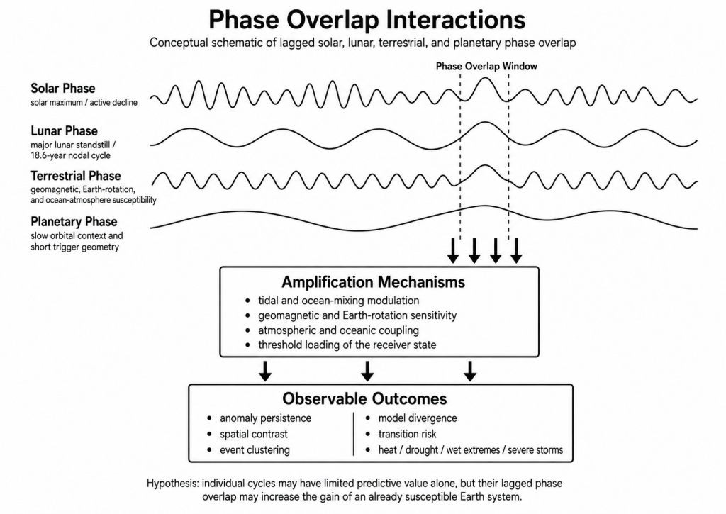
This paper proposes and formalizes the Phase-Overlap Amplification Hypothesis (POAH): independently recognized natural cycles may have limited explanatory power when analyzed one at a time, yet their temporary phase overlap may alter the gain, persistence, spatial contrast, and transition probability of an already loaded Earth system. The hypothesis is motivated by a specific multiscale configuration: the 2024-2025 major lunar standstill and 18.61-year nodal-tide maximum, the October 2024 maximum of Solar Cycle 25 and continuing elevated solar activity through 2026, measurable lunar and intradecadal terms in Earth rotation, a proposed multidecadal inner-core rotation state change, and a high-load ocean-atmosphere receiver characterized by exceptional ocean heat, evolving ENSO conditions, regional soil-moisture contrasts, and strong atmospheric moisture availability. January 2026 also contained a shorter perihelion-Jupiter-opposition geometry that can be retained as a low-weight exploratory timing variable. None of these observations, individually or jointly, proves a causal influence on weather.

The novel claim is narrower and testable: when predefined solar, lunar, terrestrial, and optional planetary phase variables overlap, and when the ocean-atmosphere receiver is already near a high-load state, the rate and persistence of compound atmospheric anomalies should exceed that predicted by conventional baseline models using greenhouse forcing, ENSO, ocean heat content, volcanic aerosols, land-surface conditions, and established modes of internal variability alone. The expected response is not required to have a fixed sign. The same overlap may amplify heat and drought in one region while increasing precipitation, severe convection, or storm persistence elsewhere. The principal outcome is therefore defined as anomaly magnitude, duration, clustering, spatial contrast, and model residual—not global temperature alone.

The paper develops a circular-phase representation for each cycle, a lagged Phase-Overlap Amplification Index, a receiver-susceptibility term, a residual-divergence measure, and a threshold transition model. It specifies historical and prospective datasets, matched-control windows, red-noise and surrogate tests, distributed-lag nonlinear models, wavelet coherence, event-coincidence analysis, out-of-sample validation, and explicit falsification criteria. The planetary term is assigned exploratory status and must improve predictive skill independently to remain in the model. If high phase-overlap conditions do not produce statistically elevated compound-anomaly behavior across repeated windows, or if the model fails to outperform conventional baselines out of sample, the hypothesis is falsified.

---

Hypothesis Statement

Hypothesis Title

The Phase-Overlap Amplification Hypothesis: Multiscale Phase Convergence as a Conditional Amplifier of Earth-System Anomaly Clustering

System Type / Domain

Coupled Sun-Earth-Moon system; heliophysics; geophysics; ocean-atmosphere dynamics; climate variability; severe-weather and hydrological extremes.

System Under Analysis

The bounded system includes the Sun, the Moon’s orbit and tidal modulation, Earth’s rotation and geomagnetic state, the ocean-atmosphere receiver, land-surface memory, and selected planetary geometries treated as candidate timing variables. The primary response domain is Earth’s atmosphere-ocean system. The proposed mechanism is not direct deterministic control of weather by planets. It is conditional amplification through phase overlap, lag, receiver susceptibility, and nonlinear threshold behavior.

Structural Model

The model treats the Earth system as a set of coupled oscillatory and slowly varying processes. Each process has a phase, amplitude, uncertainty, and pathway into the receiver. When several phases approach predefined target sectors at the same time, the system’s effective structural pressure may rise. If the receiver is already loaded by high ocean heat content, moisture, unstable circulation, low soil-moisture margin, or strong climate-mode transitions, small periodic contributions may become more visible through nonlinear interaction.

Variables Measured

1. Lunar nodal phase and tidal constituent modulation.
2. Solar-cycle phase, sunspot number, F10.7 flux, ultraviolet output, flare and CME activity, solar-wind and geomagnetic indices.
3. Earth-rotation variables, including length of day, atmospheric angular momentum, oceanic angular momentum, polar motion, and selected geomagnetic secular-variation indices.
4. Inner-core rotation-state indicators, treated cautiously because direct continuous measurement is unavailable.
5. Planetary heliocentric geometry and solar-system barycentric variables, treated as exploratory.
6. Receiver-state variables: ocean heat content, sea-surface temperature, ENSO, PDO, AMO, MJO, soil moisture, precipitable water, snow and sea-ice state, stratospheric circulation, and volcanic aerosol forcing.
7. Atmospheric outcomes: temperature and precipitation departures, extreme-event frequency, duration, area, clustering, blocking persistence, severe-convective reports, tropical cyclone activity, drought-flood contrast, and baseline-model residuals.

---

1. Hypothesis Definition

1.1 Scientific Claim

The Phase-Overlap Amplification Hypothesis states:

The coupled Earth system accumulates measurable structural pressure when several independently defined solar, lunar, terrestrial, and optional planetary phase variables enter overlapping target sectors while the ocean-atmosphere receiver is already in a high-susceptibility state. Above a critical overlap-pressure threshold, the probability of a detectable transition increases. The transition may appear as persistent circulation reorganization, increased compound-anomaly clustering, elevated model residuals, or a new quasi-stable regional pattern. If repeated high-overlap windows do not produce these outcomes at rates exceeding matched controls and conventional baseline-model expectations, the hypothesis is false.

The claim does not state that astronomical geometry determines individual tornadoes, floods, heat waves, earthquakes, or solar eruptions. It does not state that every overlap produces disaster. It does not require all regions to respond in the same direction. It predicts a change in conditional probability and system gain, not deterministic event timing.

1.2 Primary Novel Observation

Most solar-climate, lunar-climate, Earth-rotation, and planetary-timing studies test one oscillation against one outcome. That design can miss a conditional relationship in which weak or moderate inputs become detectable only when their phases overlap, the response is delayed, and the ocean-atmosphere receiver is already close to a threshold.

The primary novel observation is therefore not a fixed long-period recurrence. It is a general phase-state proposition:

Do multiple oscillatory phases become predictively important only when they overlap, after physically plausible lags, and in the presence of a susceptible terrestrial receiver?

This formulation produces a larger and more rigorous test set. Every lunar nodal cycle, solar cycle, Earth-rotation oscillation, geomagnetic transition, planetary geometry, and receiver-state transition can be evaluated. It also allows close-overlap periods, weak-overlap periods, and high-receiver-load periods to be compared without selecting only famous historical events.

1.3 Transition Definition

For this paper, a structural transition is any preregistered change satisfying at least one of the following:

1. A statistically significant regime shift in circulation, ocean state, or climate index.
2. A sustained increase in the frequency, magnitude, duration, or spatial area of compound atmospheric anomalies.
3. A significant increase in residual error after a conventional baseline model has accounted for known drivers.
4. A coherent lead-lag sequence across at least three independent observational domains.
5. A reorganization in which regional anomaly signs differ but total spatial contrast and persistence rise.

The transition requirement applies across repeated windows, not as an absolute rule for every individual overlap. A stochastic Earth system may fail to express an outcome in one window. The hypothesis is tested by whether the conditional distribution changes reliably across many windows and datasets.

---

2. THD Framework and Theoretical Model

Triune Harmonic Dynamics describes transformation through three recurring states: Emergence, Contrast, and Integration. In this paper, THD is used as a structural hypothesis framework, not as a substitute for conventional physics or evidence.

THD phase	Earth-system interpretation	Measurable expression
Base / Emergence	Background oscillators approach target phase sectors while receiver load rises	Increasing phase proximity, ocean heat, moisture, land-surface memory, or circulation predisposition
Pressure / Contrast	Multiple drivers overlap and interact with a constrained receiver	Higher anomaly variance, stronger gradients, model divergence, event clustering, circulation persistence
Integration / Transition	The system resolves accumulated pressure through reorganization	Regime shift, new circulation state, ocean-atmosphere adjustment, event release, or return toward baseline

2.1 Emergence Phase

The emergence phase begins before visible extremes. The relevant signal is not a single event but a gradual reduction in margin. Examples include increasing ocean heat content, a transition in ENSO, persistent soil-moisture deficits, unusually high precipitable water, an active solar background, or tidal-mixing phases capable of slowly altering ocean density and heat transport.

2.2 Contrast Phase

Contrast occurs when gradients sharpen and formerly separable processes begin to interact. This phase may present as simultaneous heat and drought in one region, excessive rainfall in another, severe-convective clustering along the boundary, and increased forecast uncertainty. The key prediction is not uniform warming or cooling. It is greater structural contrast and persistence.

2.3 Integration Phase

Integration is the system’s transition into a new temporary organization. Examples include a completed ENSO transition, a persistent blocking pattern, a reconfigured storm track, a basin-scale sea-surface-temperature pattern, or a release of accumulated geomagnetic or atmospheric stress. Integration may reduce pressure, but it can also establish a new baseline from which another cycle begins.

2.4 Why Phase Overlap Is Distinct From Simple Periodicity

Simple periodicity asks whether one variable repeats at a fixed interval. Phase-overlap analysis asks whether the relative positions of several cycles create windows in which their interaction terms become important. Two cycles may each have weak marginal effects yet produce a larger conditional effect when both are near selected phases. A third variable may determine whether the overlap is amplified, damped, or invisible.

This is analogous to weakly coupled oscillators in nonlinear dynamics: phase synchronization can occur without identical amplitudes, and noise can obscure the relationship unless phase and timing are analyzed directly. The proposed Earth-system application must nevertheless demonstrate statistical and physical coherence rather than relying on visual resemblance.

---

3. System Definition

3.1 System Boundaries

The primary boundary is the coupled atmosphere-ocean-land-cryosphere system from 1850 to the present, with extensions into proxy records where adequate dating and uncertainty estimates exist. External and boundary-condition inputs include solar radiation and eruptive activity, lunar tidal modulation, volcanic aerosols, greenhouse forcing, and optional planetary geometry. Internal modes include ENSO, PDO, AMO, MJO, QBO, polar vortex variability, atmospheric angular momentum, ocean circulation, and land-surface feedback.

The analysis excludes claims of astrology, symbolic planetary meaning, or direct intention. Planetary variables are limited to calculated mass, distance, angular position, barycentric motion, tidal potential, or defined geometric relations.

3.2 Interactions

Potentially plausible pathways are ranked by evidentiary status.

Tier 1: Established pathways

• Lunar gravity modulates ocean tides and solid-Earth tides.
• The 18.61-year nodal cycle changes diurnal and semidiurnal tidal constituents.
• Solar activity affects the magnetosphere, ionosphere, thermosphere, radio propagation, satellite drag, and geomagnetically induced currents.
• Atmospheric and oceanic angular momentum alter Earth rotation and polar motion.
• ENSO, ocean heat, soil moisture, and greenhouse forcing materially affect weather and climate extremes.

Tier 2: Supported but regionally or mechanistically incomplete pathways

• Nodal tidal modulation may alter ocean mixing, intermediate-water formation, steric sea level, heat transport, and regional climate variability.
• Changes in Earth rotation and deep-Earth dynamics may covary through angular-momentum exchange.
• Solar ultraviolet variability and energetic-particle effects may influence stratospheric chemistry and circulation under some conditions.

Tier 3: Exploratory pathways

• Planetary geometry may weakly modulate solar activity or provide a phase marker for solar inertial motion.
• Predefined planetary angular geometries may act as low-prior timing variables, but only if they add independent predictive value.
• Weak forcings may become detectable only near nonlinear thresholds.

Tier 3 variables are retained only if they add robust out-of-sample skill after correcting for multiple testing and red-noise bias.

3.3 Observables and Measurement Methods

Domain	Observable	Preferred source or method
Lunar	Nodal longitude, lunar declination, K1/O1/M2 modulation, perigean phase	JPL Horizons, IERS conventions, harmonic tide models
Solar	Sunspot number, F10.7, TSI, UV, flare/CME counts, solar-wind speed, IMF Bz	SILSO, NOAA SWPC, NASA/ESA archives
Geomagnetic	Kp, Ap, aa, Dst/SYM-H, auroral electrojet indices	GFZ, ISGI, WDC Kyoto, NOAA
Earth rotation	LOD, UT1-UTC, polar motion, AAM, OAM	IERS EOP C04, USNO, reanalysis angular-momentum products
Core	Differential rotation proxies and turning-point estimates	Peer-reviewed repeated-earthquake studies; no interpolation beyond evidence
Planetary	Heliocentric longitude, conjunction/opposition, barycentric angular momentum, tide-generating potential	JPL Horizons and reproducible orbital calculations
Ocean	SST, ocean heat content, mixed-layer depth, steric sea level, circulation indices	ERSST, HadSST, Argo, ORAS, EN4, altimetry, tide gauges
Atmosphere	Reanalysis fields, blocking, jet latitude, precipitable water, CAPE, shear, storm tracks	ERA5, NOAA/NCEP, JRA-55, 20CRv3
Extremes	Heat, precipitation, drought, tornadoes, floods, tropical cyclones	NOAA NCEI, SPC, IBTrACS, GHCN, GPCC, EM-DAT with reporting corrections

---

4. Prior Evidence and Historical Structural Transitions

4.1 Lunar Nodal Modulation Is Measurable

The lunar nodal cycle is not hypothetical. The Moon’s ascending node regresses over approximately 18.61 years, changing maximum lunar declination and modulating tidal constituents. Published oceanographic work reports approximately 11% modulation for K1 and 19% for O1 in equilibrium-tide formulations, with smaller but still important modulation of M2. The physical expression varies geographically because local bathymetry, resonance, and amphidromic structure alter the tidal response.

Several peer-reviewed studies provide a foundation for testing a broader overlap model:

• Yasuda and colleagues proposed that nodal modulation of strong tidal mixing near the Kuril Islands could alter North Pacific intermediate water, boundary currents, heat transport, sea-surface temperature, and the Aleutian Low.
• McKinnell and Crawford reported a statistically detectable 18.6-year signal in long northeast-Pacific air and sea-temperature records while noting that atmospheric circulation explained substantial recent variability.
• Hasumi and colleagues modeled a pathway from localized tidal mixing to ENSO-like Pacific variability.
• Yasuda identified an 18.6-year periodicity in a tree-ring reconstruction of the Pacific Decadal Oscillation and reported phase-dependent lags.
• Osafune and Yasuda found bidecadal variations in Bering Sea water masses synchronized with nodal tidal modulation.
• Peng and colleagues used records from 574 tide gauges and found that nodal modulation can change monthly high-water levels by up to approximately 30 cm at some locations.
• Bult and colleagues reported an 18.6-year steric sea-level signal along western Europe, interpreted as a possible ocean-mixing response in the upper 400 m.

These findings do not establish a global weather-control mechanism. They demonstrate that the lunar nodal cycle can enter ocean and coastal systems through measurable pathways, often with regional phase differences and lags.

4.2 Solar Phase Is a Conditional Gate

Solar Cycle 25 reached its smoothed maximum in October 2024 with a sunspot number near 161, according to WDC-SILSO. Solar activity remained capable of producing complex active regions and strong flares into 2026. The solar contribution to lower-atmosphere variability is expected to be small relative to greenhouse forcing and internal climate variability, but solar phase is directly relevant to space weather and may operate as a conditional gate in a broader overlap model.

Historical geomagnetic events show why phase alone is insufficient. The Carrington Event occurred in September 1859, several months before the February 1860 maximum of Solar Cycle 10. The May 1921 superstorm occurred during the declining phase of Solar Cycle 15 and reached an estimated intensity comparable to Carrington, demonstrating that major events are not confined to the exact sunspot maximum. The March 1989 storm occurred near the maximum of Solar Cycle 22 and caused the Quebec grid collapse. Thus, the appropriate variable is a continuous solar activity and eruptive-potential state rather than a binary maximum-year flag.

4.3 Earth Rotation Contains Lunar and Intradecadal Signals

USNO and IERS documentation identify an 18.6-year periodic term in length of day produced by solid-Earth tides, along with annual, semiannual, fortnightly, and monthly terms. Irregular length-of-day variations on approximately five- to fifteen-year timescales are associated with processes in the atmosphere, oceans, and deep Earth. This establishes a measurable bridge between astronomical forcing and terrestrial angular momentum.

Recent studies have reported an approximately 8.5-year inner-core wobble signal in polar motion and length of day. Other work has proposed a roughly seven-decade oscillation in differential inner-core rotation, with a recent near-pause or turning point. These results are scientifically active and not fully settled. They justify including Earth-rotation and deep-Earth proxy variables, but they do not justify a simple statement that a slowing core weakens the magnetosphere or directly causes weather extremes.

4.4 Planetary Geometry Is Measurable but Physically Unresolved

Planetary positions and angular relationships can be calculated precisely from ephemerides. Relevant candidate variables include Sun-Earth-planet elongation, opposition and conjunction angles, heliocentric angular separations, solar-system barycentric displacement, and the rate at which those geometries form and dissolve. The January 2026 perihelion-Jupiter-opposition sequence is one example of a short, predefined geometric interval that can be tested without assuming a causal effect.

The physical interpretation remains disputed. Historical papers have proposed links between planetary motion, solar inertial motion, and solar periodicities. Other studies have found that apparent spectral matches can arise from red noise, frequency-bin selection, filtering choices, and multiple testing. Direct planetary tides on the Sun and Earth are generally very small compared with internal solar dynamics and lunar-solar terrestrial tides. Planetary geometry is therefore not part of the core causal model. It remains a low-prior candidate timing or interaction variable and must be removed if it adds no independent out-of-sample skill.

4.5 Preliminary 2026 Outcome Pattern

By June 2026, NOAA reported several relevant observations:

• The globe experienced its second-warmest June in the instrumental record, while global ocean surface temperature was the warmest on record for June.
• The western and southwestern United States had their warmest January-June period on record and received less than 70% of average precipitation.
• June produced 374 preliminary U.S. tornado reports, with Illinois, Indiana, and Missouri setting state records for June reports.
• Precipitation was unusually high across parts of the Plains, Midwest, Great Lakes, and Hawaii, while much of the West and sections of the East Coast remained dry.
• El Nino emerged and strengthened rapidly during summer 2026, providing a strong conventional explanation for part of the evolving ocean-atmosphere pattern.

These observations are not confirmation of POAH. They establish a prospective test period and illustrate the predicted sign-changing structure: heat and drought, excessive precipitation, and severe convection can coexist in different parts of the same system.

---

5. Historical Phase-Overlap Windows

A strong test cannot rely on a few selected disasters. The confirmatory dataset should include every calculable phase window. Nevertheless, several windows illustrate the model’s logic and its need for negative controls.

5.1 Approximate Lunar Diurnal-Tide Maxima and Nearest Solar Maxima

Using 1969 as a published diurnal nodal-tide maximum and stepping by 18.613 years produces the following approximate sequence. Solar maxima are from WDC-SILSO. Values are rounded and should be replaced by exact astronomical phase calculations in the final analysis.

Approximate lunar maximum	Nearest solar maximum	Absolute separation	Preliminary classification
1857.3	1860.2	2.8 years	Post-standstill active solar rise; Carrington in 1859
1875.9	1870.7	5.3 years	Weak solar-lunar overlap; useful control
1894.5	1894.1	0.5 years	Strong temporal overlap
1913.2	1917.7	4.5 years	Lunar maximum near solar minimum; useful control
1931.8	1928.3	3.5 years	Moderate separation
1950.4	1947.4	3.0 years	Moderate separation before strong Cycle 19
1969.0	1968.9	0.1 years	Very close solar-lunar overlap
1987.6	1989.9	2.3 years	Post-lunar peak, rising toward solar maximum
2006.2	2001.9	4.4 years	Weak overlap; negative-control candidate
2024.8	2024.8	less than 0.1 years	Exceptionally close solar-lunar overlap

This table shows that exact solar-lunar coincidence is uncommon but not unique. The hypothesis must therefore explain why some close overlaps produce stronger atmospheric expressions than others. Receiver state, terrestrial phase, regional ocean geometry, season, and lag are essential discriminators.

5.2 Historical Phase-Overlap Window, 1857-1860

The lunar nodal maximum preceded the Carrington Event by roughly two years, while Solar Cycle 10 was rising toward its 1860 maximum. The event itself was a heliophysical and technological transition, not a demonstrated weather event. Its value to this hypothesis is that it shows a high solar-response outcome within a post-nodal, active-solar window.

The 1857-1860 window should be evaluated using reconstructed sunspots, auroral reports, geomagnetic records, pressure and temperature observations, ship logs, storm tracks, and volcanic-aerosol controls. The Carrington Event cannot be counted as evidence for atmospheric amplification unless atmospheric variables independently show the predicted structure.

5.3 1894-1895 Window

The approximate lunar diurnal-tide maximum and Solar Cycle 13 maximum were separated by about half a year. This is a critical historical test because it offers a close phase overlap without the fame of Carrington. If POAH is valid, some combination of oceanic, atmospheric, geomagnetic, or residual-anomaly indicators should rise relative to matched controls. If no such signal exists, the result weighs against a simple solar-lunar overlap model and increases the importance of receiver and terrestrial-state terms.

5.4 1968-1970 Window

The 1969 nodal maximum and November 1968 solar maximum were nearly coincident. Modern reanalysis, satellite-era observations, tide gauges, radiosonde data, storm archives, and improved geomagnetic indices make this one of the strongest retrospective test periods. The analysis should quantify—not narratively select—temperature, precipitation, blocking, tropical cyclones, severe weather, ocean heat transport, and geomagnetic disturbance from 1967 through 1971.

5.5 1987-1990 Window

The nodal maximum occurred approximately two years before the November 1989 solar maximum. The March 1989 geomagnetic storm and Quebec blackout occurred within this rising-overlap interval. This supports the relevance of solar activity to technological susceptibility, but it does not establish an atmospheric effect. The window is valuable because modern reanalysis and ocean data are extensive.

5.6 2005-2008 Window as a Negative Control

The 2006 nodal maximum occurred several years after the 2001 solar maximum and before the deep 2008-2009 solar minimum. If the overlap model is correct, this period should generally have a lower solar-lunar overlap score than 1969 or 2024. Atmospheric anomalies may still occur because ENSO, greenhouse forcing, volcanic activity, or internal variability can generate extremes independently. The model succeeds only if its index improves conditional prediction, not if it labels every extreme as astronomical.

5.7 2024-2027 Prospective Window

The current period combines an unusually close solar-lunar phase overlap, ongoing active solar conditions, a rapid ENSO transition, record-warm ocean conditions, and a proposed terrestrial rotation/core transition context. It is therefore a preregisterable prospective window. The January 2026 perihelion-Jupiter-opposition geometry is retained only as a lower-confidence nested timing variable.

---

6. Structural Pressure Measurement

The hypothesis requires outcomes that distinguish ordinary variability from a high-gain state.

6.1 Anomaly Frequency

For each grid cell and region, count days or months exceeding the 90th, 95th, and 99th percentiles of temperature, precipitation, wind, CAPE, precipitable water, drought severity, or storm intensity. Percentiles must be calculated relative to a moving or detrended baseline to avoid treating long-term warming alone as phase-overlap evidence.

6.2 Duration and Persistence

Measure consecutive-event duration, blocking duration, heat-wave length, drought persistence, wet-spell duration, and autocorrelation time. POAH predicts that overlap windows may increase persistence even when the monthly mean is not exceptional.

6.3 Spatial Area and Contrast

Calculate the fraction of a region exceeding anomaly thresholds and a spatial-contrast measure such as the standard deviation or gradient of standardized anomalies across predefined climate regions. A high-contrast month may contain simultaneous drought and flood without a large national mean anomaly.

6.4 Clustering

Use event-coincidence analysis, scan statistics, and point-process models to test whether severe events occur more closely in time or space than expected under matched seasonal baselines. Tornado-report data require correction for population, radar coverage, reporting practice, and preliminary-report duplication.

6.5 Volatility and Regime Instability

Track rolling variance, entropy, transition probability between circulation regimes, forecast ensemble spread, and the frequency of rapid reversals. A system near a threshold may show greater instability before settling into a new state.

6.6 Model Divergence

Define divergence as the residual between observed behavior and a baseline model containing established climate drivers. The hypothesis is strongest when overlap predicts the residual, not when it simply recapitulates ENSO or the seasonal cycle.

---

7. Structural Pressure Sources and Independent Variables

Let the candidate drivers be standardized to comparable ranges.

• x1: Lunar nodal phase. Exact nodal longitude, maximum declination, and local tidal-constituent modulation.
• x2: Solar activity state. Continuous combination of smoothed sunspot number, F10.7, UV, flare/CME occurrence, solar wind, and geomagnetic response.
• x3: Earth-rotation state. Detrended LOD residual, AAM, OAM, and polar-motion phase after removing modeled tides.
• x4: Geomagnetic state. Secular field strength, aa/Ap/Kp/Dst activity, and rate-of-change measures.
• x5: Deep-Earth proxy state. Published inner-core differential-rotation or wobble estimates, with broad uncertainty bands.
• x6: Planetary geometry. Reproducible heliocentric or barycentric metrics. Exploratory only.
• x7: Ocean receiver load. Ocean heat content, SST pattern, mixed-layer depth, and thermocline state.
• x8: Atmospheric receiver load. ENSO, MJO, QBO, blocking, jet latitude, precipitable water, stratospheric state.
• x9: Land-surface load. Soil moisture, snow cover, vegetation stress, drought, and surface-energy partitioning.
• x10: External controls. Greenhouse forcing, volcanic aerosol optical depth, anthropogenic aerosols, and long-term trend.

The core hypothesis concerns x1 through x5 interacting with x7 through x9. x6 is removable. x10 belongs in the baseline and is not optional.

---

8. Phase-Overlap Structural Equation

8.1 Circular Phase Representation

For cycle i with period Ti and reference epoch t0,i:

[\theta_i(t)=2\pi\left[\frac{t-t_{0,i}}{T_i}\bmod 1\right]]

A target phase mi is defined before outcome inspection. Phase proximity is represented by a circular kernel:

[a_i(t)=\frac{\exp\left[\kappa_i\cos(\theta_i(t)-\mu_i)\right]-\exp(-\kappa_i)}{\exp(\kappa_i)-\exp(-\kappa_i)}]

where ai ranges approximately from 0 to 1 and kappa controls the width of the target sector. A broad kappa represents a wide physical window; a narrow kappa represents a precise phase requirement.

8.2 Lagged Phase Variables

Because ocean and atmospheric responses may be delayed, each phase term may enter with a preregistered lag tau_i:

[a_i^*(t)=a_i(t-\tau_i)]

The confirmatory lunar lag will be tested over 12-30 months, with an exploratory range of 0-36 months. Solar and geomagnetic lags may be hours to months depending on the outcome. Ocean-circulation pathways may require multiple years.

8.3 Receiver Susceptibility

Define a receiver index R(t) from variables measured before the outcome window:

[R(t)=\sigma\left(\alpha_0+\sum_{j=1}^{m} v_j z_j(t)\right)]

where sigma is the logistic function and zj includes ocean heat content, ENSO transition rate, precipitable water, soil-moisture contrast, mixed-layer anomalies, and circulation persistence. The index must not include the outcome being predicted.

8.4 Phase-Overlap Amplification Index

The principal multiplicative model is:

[H(t)=R(t)\prod_{i=1}^{n}\left[\epsilon+(1-\epsilon)a_i^*(t)\right]^{w_i}]

where H is the Phase-Overlap Amplification Index, epsilon prevents any single term from forcing the product to zero, and wi are nonnegative weights constrained to sum to one within each tier.

An interaction-regression form will also be tested:

[P(t)=\beta_0+\sum_i\beta_i a_i^(t)+\sum_{i<j}\gamma_{ij}a_i^(t)a_j^*(t)+\eta H(t)]

The hypothesis predicts that interaction terms and H(t) add more out-of-sample skill than the individual phase terms alone.

8.5 Threshold Condition

[H(t)>H_c \Rightarrow \Pr(\text{Transition within }\Delta t)\text{ increases}]

The threshold Hc is estimated in training data and frozen before testing. A transition is not required in every instance. Instead, the event rate above Hc must exceed the matched-control rate by a preregistered amount.

---

9. Model Incompleteness and Verification Gap

9.1 What Current Models Already Explain

Modern weather and climate models include radiative forcing, ocean-atmosphere dynamics, moisture, land-surface feedback, stratospheric processes, ENSO, MJO, and many other drivers. They can generate heat waves, droughts, floods, tornado environments, and storm-track changes without any planetary term. Anthropogenic warming substantially raises the baseline probability and intensity of many heat extremes and heavy-precipitation events.

A phase-overlap paper must therefore avoid claiming that anomalies unexplained in casual observation are absent from science. The verification gap is narrower:

1. Deterministic astronomical tidal modulation is often treated as a local coastal or ocean-mixing correction rather than as part of a multiscale compound-phase model.
2. Solar, lunar, Earth-rotation, and receiver variables are usually studied in separate literatures.
3. Phase relationships and lags may be lost when analyses use annual averages or fixed-sign correlations.
4. Models may search for a mean-temperature signal while the true outcome is variance, persistence, spatial contrast, or regime-transition probability.
5. Weak astronomical terms may be conditionally important only when receiver susceptibility is high.

9.2 Divergence Locations

The hypothesis should be tested where conventional models have known difficulty or large uncertainty:

• subseasonal-to-seasonal persistence;
• blocking onset and duration;
• rapid ENSO transitions;
• regional drought-flood coexistence;
• severe-convective clustering;
• compound coastal flooding;
• ocean heat redistribution and steric sea-level variability;
• extreme geomagnetic-event timing within active solar phases.

The existence of forecast error does not prove a missing astronomical variable. It identifies locations where an additional predictor can be evaluated.

---

10. Signal Divergence and Residual Error Model

Let O(t,r) be observed outcome in time t and region r. Let M0(t,r) be the prediction from a conventional baseline model.

[D(t,r)=|O(t,r)-M_0(t,r)|]

A signed residual is also retained:

[e(t,r)=O(t,r)-M_0(t,r)]

POAH predicts:

[E[D\mid H>H_c] > E[D\mid H\le H_c]]

and, more strongly, that adding H improves predictive skill:

[\text{Skill}(M_0+H)>\text{Skill}(M_0)]

The baseline model should include trend, seasonality, ENSO, PDO/AMO where appropriate, MJO, QBO, volcanic aerosol optical depth, ocean heat content, SST patterns, soil moisture, snow and sea ice, greenhouse forcing, and autoregressive structure. The phase-overlap model is not allowed to claim variance already explained by these terms.

---

11. Pre-Transition Indicators

The following indicators are preregistered as potential signs of an approaching high-gain state:

1. Rising absolute anomaly variance across multiple regions.
2. Increasing persistence of blocking, heat, wet spells, or drought.
3. Stronger spatial gradients between adjacent wet/dry or hot/cool regions.
4. Rapid shifts in atmospheric or oceanic angular momentum.
5. Increased forecast-ensemble spread followed by convergence into a persistent regime.
6. Simultaneous or sequential clustering of heat, severe convection, and heavy precipitation along circulation boundaries.
7. Accelerating ENSO transition or thermocline adjustment.
8. Nodal-phase-consistent changes in local tide range, mixing proxies, or steric sea level.
9. Elevated geomagnetic activity during an active solar phase.
10. Persistent residuals after conventional controls.

No single indicator confirms the hypothesis. Confirmation requires a reproducible multivariate pattern.

---

12. Structural Failure Location Hypothesis

Transitions should appear first where load is concentrated and slack is low.

12.1 Weakest Constraints

• Coastal regions where nodal tide modulation combines with sea-level rise and storm surge.
• Ocean straits, ridges, island arcs, and continental slopes where tidal mixing is strong.
• Power-grid regions with high ground conductivity contrast and long transmission lines.
• Agricultural regions with low soil-moisture margin.
• Urban areas with strong heat-island amplification and limited cooling redundancy.

12.2 Highest Stress Concentrations

• Boundaries between drought and moisture-rich air masses.
• Jet-stream and storm-track transition zones.
• Warm ocean regions with high atmospheric moisture flux.
• Regions undergoing rapid ENSO teleconnection adjustment.
• Geomagnetic latitudes and electrical-network geometries susceptible to induced currents.

12.3 Resonance Points

Local resonance is expected to matter more than global average forcing. Tidal response depends on basin geometry. Atmospheric response depends on topography, land-sea contrast, jet position, and background climate. The same astronomical phase can therefore produce different regional signs and amplitudes.

---

13. Predicted Structural Outcomes

If overlap pressure rises, the Earth system may resolve through one or more of the following:

1. A detectable circulation regime shift.
2. Increased frequency or duration of compound extremes.
3. Stronger regional contrast between drought and excess precipitation.
4. Enhanced coastal high-water risk in nodally sensitive regions.
5. Ocean mixing and heat-transport anomalies with multiyear propagation.
6. Elevated model residuals concentrated in specific lags after phase maxima.
7. Technological disruption if elevated solar activity produces Earth-directed eruptions.
8. Model revision if phase-overlap terms consistently add predictive skill.
9. Rejection of the planetary component if it adds no independent skill.
10. Rejection of the full hypothesis if no repeatable conditional amplification is found.

---

14. Transition Likelihood Model

A logistic event model is proposed:

[\Pr(Y_{t,r}=1)=\sigma\left(\alpha_r+\lambda_t+\beta H(t)+\mathbf{c}^{\mathsf T}\mathbf{X}_{t,r}\right)]

where alpha_r is a regional effect, lambda_t controls trend and seasonality, X contains conventional predictors, and Y indicates a transition or extreme cluster.

For continuous outcomes:

[Y_{t,r}=f(\mathbf{X}{t,r})+g(H(t),\tau)+u_r+e{t,r}]

where g is estimated with a distributed-lag nonlinear model. The key test is whether g is stable, interpretable, and out-of-sample predictive.

---

15. Methods and Statistical Test Plan

15.1 Preregistration

Before outcome testing, register:

• cycle definitions and reference epochs;
• target phase sectors and widths;
• acceptable lag ranges;
• core and exploratory variables;
• regions and outcome metrics;
• baseline model specification;
• missing-data rules;
• significance thresholds;
• model-selection penalties;
• prospective forecast windows.

The planetary term cannot be tuned after viewing outcomes.

15.2 Data Periods

Three nested periods are recommended:

1. Modern high-quality period, 1979-present: satellite era, ERA5, robust SST, storm, and solar data.
2. Instrumental extension, 1850-present: temperature, precipitation, sunspots, aa index from 1868, tide gauges, 20CRv3, historical storm archives.
3. Proxy extension: tree rings, speleothems, ice cores, documentary records, and cosmogenic isotopes, with dating uncertainty explicitly modeled.

15.3 Wavelet Coherence

Cross-wavelet transform and wavelet coherence can identify time-localized relationships between phase variables and geophysical outcomes. Significance must be tested against red-noise and phase-randomized surrogates. The cone of influence, smoothing choices, and degrees of freedom must be reported. A spectral peak near 18.6 years is not sufficient if it is unstable, nonstationary, or produced by filtering.

15.4 Circular Statistics

Use Rayleigh, Kuiper, or Watson tests to determine whether extremes cluster in particular cycle phases. Correct for seasonality and serial dependence. When testing many periods or phase sectors, use preregistration or false-discovery-rate correction.

15.5 Distributed-Lag Nonlinear Models

DLNMs are appropriate because effects may be nonlinear and delayed. They can estimate an exposure-lag-response surface for lunar phase, solar state, or overlap index while controlling conventional predictors. Critical windows should be confirmed in held-out data.

15.6 Event-Coincidence Analysis

Define extremes as threshold events and test whether they occur within specified lags after high-overlap intervals more often than expected under stochastic point-process null models. This approach is useful for severe storms, floods, geomagnetic disturbances, and abrupt regime transitions.

15.7 Matched Controls

Each high-overlap month should be matched to control months with similar:

• season;
• long-term warming level;
• ENSO state;
• ocean heat content;
• volcanic aerosol state;
• land-surface conditions;
• data quality and reporting coverage.

The comparison isolates overlap from known background drivers.

15.8 Additive Versus Interaction Models

Compare:

1. baseline only;
2. baseline plus individual phase terms;
3. baseline plus pairwise interactions;
4. baseline plus full overlap index;
5. baseline plus overlap index excluding planetary variables.

The hypothesis requires models 3 or 4 to outperform model 2. If individual terms explain the result without interaction, the phase-overlap claim is weakened.

15.9 Out-of-Sample Validation

Use blocked time-series cross-validation. Do not randomly shuffle individual months, which leaks temporal information. Possible splits include:

• train 1850-1950, test 1951-2025;
• train 1979-2005, test 2006-2025;
• leave-one-nodal-cycle-out validation;
• leave-one-region-out validation.

Metrics may include RMSE, MAE, CRPS, Brier score, log score, area under the precision-recall curve, and event-rate ratios.

15.10 Surrogate and Null Tests

Required nulls include:

• red-noise surrogate phase series;
• phase-randomized outcomes preserving spectrum;
• randomly shifted cycle reference epochs;
• alternative periods scanned over the same range;
• placebo planetary bodies or synthetic geometries;
• seasonally matched random windows;
• negative-control outcomes with no plausible pathway.

The overlap model must beat the distribution generated by these nulls.

---

16. Prospective Observation Protocol: August 2026-May 2027

The following observation protocol is prospective. Its dates, variables, thresholds, and failure conditions should be frozen before the monitoring period is evaluated. The purpose is not to predict a particular disaster. It is to determine whether a high phase-overlap state is followed by measurable increases in anomaly magnitude, persistence, clustering, spatial contrast, or residual error beyond conventional Earth-system models.

16.1 Locked Observation Window

The primary monitoring window is August 1, 2026 through May 31, 2027. This interval spans late-summer heat and tropical activity, the autumn circulation transition, the boreal winter ENSO and stratospheric response, and the following spring severe-weather and hydrological transition.

No event occurring outside this interval may be moved into the confirmatory test after the fact. Exploratory lead and lag analyses may extend six months on either side, but those results must be reported separately and corrected for the expanded search.

16.2 Required Monitoring Streams

Domain	Variables to record	Minimum frequency	Primary source class	Test purpose
Solar	Sunspot number, F10.7 flux, M- and X-class flare counts, Earth-directed CME speed, solar-wind speed and density, IMF Bz, proton events	Daily, summarized by 27-day solar rotation and month	SILSO, NOAA SWPC, NASA/ESA catalogs	Measure solar activity, recurrent active regions, and actual Earth-directed forcing rather than solar-cycle phase alone
Geomagnetic	Kp, Ap, aa, Dst or SYM-H, auroral electrojet indices, magnetopause-compression events	Hourly to daily	NOAA, WDC Kyoto, GFZ, ESA	Identify whether solar forcing produces clustered terrestrial magnetic responses
Lunar and tidal	Lunar nodal phase, declination extrema, perigee/apogee, syzygy, K1/O1/M2 nodal modulation, local predicted and observed high water	Event, daily, and monthly	JPL Horizons, NOAA tides, national hydrographic agencies	Distinguish the slow nodal envelope from ordinary monthly and fortnightly tidal forcing
Earth orientation	Length-of-day residuals after conventional tidal correction, UT1-UTC, polar motion, atmospheric angular momentum, oceanic angular momentum	Daily to monthly	IERS, USNO, ECMWF/NCEP AAM, ocean angular-momentum products	Test whether angular-momentum exchange or terrestrial phase changes precede atmospheric reorganization
Geomagnetic secular state	Field intensity and secular variation at observatories, geomagnetic jerks or acceleration changes where available	Monthly to quarterly	INTERMAGNET, IGRF/WMM updates, peer-reviewed core-field products	Evaluate the terrestrial-state term without assuming that core behavior directly causes weather
Planetary geometry	Predefined Sun-Earth-Jupiter and other selected angular indices, barycentric variables, angle-formation and decay rates	Daily, aggregated monthly	JPL Horizons	Low-prior exploratory test; retain only if it adds independent predictive value
Ocean receiver	Upper-ocean heat content, SST anomaly fields, marine heatwave area, thermocline depth, steric sea level, ENSO, PDO, AMO, tropical Atlantic and Indian Ocean indices	Weekly to monthly	NOAA, NASA, Copernicus, Argo, Hadley Centre	Quantify background heat, stored energy, and oceanic memory
Atmospheric receiver	Precipitable water, CAPE, vertical wind shear, jet latitude and speed, blocking, MJO, QBO, stratospheric polar-vortex strength, atmospheric rivers	Daily to weekly	ERA5, NCEP, NOAA CPC, ECMWF	Measure the state that determines the sign and location of weather expression
Land receiver	Soil moisture, evapotranspiration, snow cover, snow-water equivalent, vegetation stress, drought indices	Weekly to monthly	NOAA, NASA GRACE/SMAP, USDA, national hydrological services	Measure land-memory and surface-amplification pathways
Weather outcomes	Temperature and precipitation percentiles, heatwave duration, cold outbreaks, tornado and hail clustering, tropical cyclone intensity, flood and drought area, coastal high-water events	Daily, event, and monthly	NOAA/NCEI, SPC, IBTrACS, national agencies	Test anomaly magnitude, duration, clustering, and spatial contrast
Model divergence	Residuals from preregistered seasonal and subseasonal baseline models; forecast bust frequency; spread-error ratio	Weekly to monthly	ECMWF, NOAA, ensemble hindcasts and forecasts	Determine whether known models lose skill during high-overlap intervals

16.3 Seasonal Observation Blocks

Block A: August-October 2026 – Warm-Season Persistence and Transition

Monitor:

1. Persistence or re-expansion of regional heat and drought after climatological seasonal decline.
2. Marine heatwave area and upper-ocean heat-content anomalies in the North Atlantic, tropical Pacific, Gulf of Mexico, and western boundary-current regions.
3. Tropical cyclone rapid intensification, track clustering, rainfall efficiency, and compound coastal flooding.
4. Heavy-precipitation clustering near sharp wet-dry boundaries.
5. Severe-convective outbreaks occurring outside normal regional or seasonal concentration.
6. Jet-stream persistence, blocking, monsoon withdrawal timing, and abrupt circulation transitions.
7. Clusters of Earth-directed CMEs or geomagnetic storms separated by approximately one solar rotation.
8. Forecast residuals that persist across successive model cycles rather than isolated forecast errors.

Block B: November 2026-January 2027 – Ocean-Atmosphere and Stratospheric Integration

Monitor:

1. ENSO amplitude, location, and teleconnection strength relative to conventional expectations.
2. North Pacific and North Atlantic pressure-pattern persistence, including blocking and storm-track displacement.
3. Stratospheric polar-vortex strength, sudden-stratospheric-warming precursors, and downward coupling.
4. Atmospheric-river frequency, integrated vapor transport, and repeated landfall corridors.
5. Warm-cold spatial contrast, especially simultaneous regional extremes rather than a single hemispheric mean.
6. Coastal high-water events where nodal modulation, storm surge, waves, and sea-level anomaly combine.
7. AAM/OAM and LOD shifts coincident with major circulation reorganizations.
8. Energy-system stress only as a secondary impact indicator, not as evidence of astronomical causation.

Block C: February-May 2027 – Hydrological Release and Spring Transition

Monitor:

1. Snowpack, soil-moisture, river-storage, and flood-potential accumulation before spring melt.
2. Spring temperature volatility, early heat episodes, late freezes, and rapid transitions between them.
3. Tornado, hail, and severe-convective clustering after adjustment for reporting density and radar coverage.
4. Repeated heavy-rain corridors, flash-flood clusters, and drought-to-flood transitions.
5. Tropical Pacific, North Pacific, and Atlantic SST reorganization and any ENSO phase change.
6. Springtime geomagnetic activity and whether magnetic disturbances cluster with independently defined solar forcing.
7. Persistence of baseline-model residuals into a second season, which would be more informative than one isolated anomalous month.
8. Whether the system returns toward ordinary variance or settles into a new quasi-stable circulation regime by May 31, 2027.

16.4 Predefined Outcome Metrics

The monitoring period should be judged using fixed metrics rather than narrative event selection:

1. Compound Anomaly Index (CAI): standardized combination of absolute temperature anomaly, absolute precipitation anomaly, event duration, affected area, and simultaneous regional contrast.
2. Persistence Index: fraction of days in a month belonging to events lasting at least seven days, with a secondary threshold of fourteen days.
3. Spatial Contrast Index: area-weighted variance of standardized temperature and precipitation anomalies across predefined regions.
4. Event Clustering Index: excess event coincidence within 7-, 14-, and 30-day windows compared with seasonally matched Poisson, negative-binomial, and block-bootstrap controls.
5. Model Divergence Index: absolute standardized residual between observations and the preregistered baseline ensemble, evaluated for persistence and cross-variable coherence.
6. Cross-Domain Transition Score: count of independent domains – ocean, atmosphere, land, geomagnetic, Earth orientation – entering their historical top decile within a 30-day interval.
7. Phase-Conditioned Risk Ratio: ratio of compound-anomaly incidence during top-decile overlap-index periods to matched low-overlap periods with similar ENSO, season, trend, and receiver state.

16.5 Prospective Support Conditions

The observation window supports POAH only if all of the following are met:

1. High phase-overlap scores precede or coincide with a statistically elevated CAI, persistence, spatial contrast, or model-divergence measure.
2. The effect appears in at least three independent observational domains and is not driven by one reporting archive.
3. Interaction models outperform the conventional baseline and single-cycle models out of sample by the preregistered skill threshold.
4. The inferred lags remain stable under leave-one-window-out and phase-randomized tests.
5. The result survives correction for ENSO, anthropogenic trend, ocean heat content, volcanic forcing, seasonality, autocorrelation, and multiple testing.

16.6 Prospective Null Conditions

The hypothesis is weakened or falsified for this window if:

1. August 2026-May 2027 is statistically ordinary after conventional controls.
2. High overlap scores do not correspond to higher anomaly magnitude, persistence, clustering, contrast, or residual error.
3. Similar or stronger results arise from randomly shifted phase epochs or arbitrary comparison periods.
4. The apparent signal depends on one famous event, one region, preliminary storm reports, or post hoc date selection.
5. Planetary terms fail to improve skill; in that case they must be removed even if the core solar-lunar-terrestrial model remains under test.

16.7 Observation and Data-Freeze Schedule

• Weekly: archive solar, geomagnetic, atmospheric-circulation, severe-weather, and forecast-residual variables.
• Monthly: calculate phase indices, receiver susceptibility, CAI, persistence, spatial contrast, and matched-control comparisons.
• Quarterly: publish a frozen interim table without changing thresholds, weights, regions, or target dates.
• May 31, 2027: close the prospective observation window.
• After final data maturation: conduct the confirmatory evaluation using quality-controlled climate, tornado, cyclone, tide-gauge, and reanalysis datasets. Preliminary reports must not be treated as final outcomes.

---

17. Observable Confirmation Signals

The hypothesis receives support only if several of the following occur:

1. Top-decile H months have a compound-extreme rate at least 20% above matched controls, with a confidence interval excluding unity.
2. The overlap model improves out-of-sample probabilistic skill by at least 5% relative to the conventional baseline across multiple regions or datasets.
3. Interaction terms remain significant after false-discovery-rate correction.
4. The inferred lunar lag is stable in a confirmatory 12-30-month range and is not merely an artifact of scanning.
5. Similar phase-response relationships appear in independent ocean, atmosphere, and Earth-rotation records.
6. The relationship survives detrending, volcanic controls, ENSO controls, and red-noise surrogates.
7. Negative-control periods such as weak solar-lunar overlaps show lower conditional anomaly rates.
8. The planetary term adds independent predictive value and survives placebo-geometry tests; otherwise it is removed without invalidating the core solar-lunar-terrestrial hypothesis.

---

18. Falsification Criteria

The core hypothesis is falsified if, after preregistration and adequate data quality:

1. High overlap scores do not predict a higher rate, magnitude, duration, or clustering of compound anomalies than matched controls.
2. Interaction models do not outperform additive individual-cycle models out of sample.
3. The apparent effect vanishes after controlling ENSO, trend, ocean heat content, volcanic aerosols, soil moisture, and established circulation modes.
4. Phase relationships are inconsistent across cycles, regions, or datasets and cannot be explained by known local tidal phase differences.
5. Equivalent or stronger results arise from randomly shifted reference epochs or arbitrary periods.
6. The 12-30-month lunar lag fails confirmatory testing and only appears after extensive post hoc scanning.
7. The model cannot predict any part of the 2026-2027 prospective window better than baseline models.
8. The overlap index fails leave-one-cycle-out validation.
9. The planetary term fails to add reproducible skill. In that case the planetary extension is falsified even if the narrower solar-lunar-terrestrial model survives.
10. Reported historical matches depend on selective event inclusion, date-window expansion, or uncorrected changes in observational coverage.

A null result is scientifically useful. It would show that the measured phase configuration is not meteorologically predictive beyond conventional controls.

---

19. Final Hypothesis Test Statement

[H(t)>H_c \Rightarrow \Pr(\text{compound Earth-system transition within }\Delta t)\text{ increases}]

If sustained high H across repeated, preregistered windows does not increase transition probability or predictive skill relative to conventional baselines and matched controls, the Phase-Overlap Amplification Hypothesis is false.

---

20. Competing Explanations

A strong paper must state what can explain the observations without POAH.

20.1 Anthropogenic Climate Change

Long-term greenhouse forcing raises ocean and air temperature, increases atmospheric moisture capacity, and shifts the probability of many extremes. This is not a competing minor factor; it is a primary baseline driver. Phase overlap, if real, would modulate variability around this changing baseline.

20.2 ENSO and Pacific Heat Redistribution

The rapid 2026 transition into El Nino provides a direct, established mechanism for global circulation and precipitation changes. Any current phase-overlap claim must add skill beyond ENSO and should not appropriate ENSO-driven anomalies as proof.

20.3 Internal Atmospheric Variability

MJO, QBO, blocking, jet variability, stratospheric sudden warmings, and stochastic weather can create clusters without astronomical phase coupling.

20.4 Volcanic Aerosols

Historical cold and wet episodes near some candidate phase-overlap windows may be dominated by volcanic forcing. Volcanic aerosol optical depth must be included in all historical models.

20.5 Observation and Reporting Bias

Tornado counts, flood losses, and historical disaster reports change with population, detection technology, communications, and record preservation. Environmental variables should be preferred over impact narratives.

20.6 Multiple Testing and Period Hunting

A dense set of astronomical periods makes accidental matches likely. The paper therefore requires preregistered periods, phase sectors, and lags, plus surrogate tests and held-out validation.

---

21. Real-World Implications

A. Domain-Level Impact

If validated, the model would add a conditional multiscale timing layer to Earth-system science. It would not replace dynamical weather and climate models. It would suggest that deterministic astronomical phases can be useful when represented as interactions with receiver susceptibility rather than as direct single-cycle forecasts.

B. Predictive Capability

The model would enable state-based window forecasting. Instead of saying an event repeats every fixed number of years, analysts would estimate when several phases and receiver loads jointly raise transition probability. This is more flexible and more falsifiable than calendar recurrence.

C. Measurement and Instrumentation

A validated model would justify development of a public Phase-Overlap Amplification Index combining:

• exact astronomical phases;
• solar and geomagnetic activity;
• Earth-rotation residuals;
• ocean and atmospheric receiver state;
• uncertainty intervals and regional phase corrections.

The index should be published with code, data versions, and frozen weights.

D. Engineering and Application Layer

Applications could include:

• coastal flood planning that incorporates nodal modulation and sea-level rise;
• seasonal risk monitoring for compound heat, drought, and precipitation;
• power-grid readiness during active solar phases;
• timing of maintenance and redundancy testing;
• agricultural planning in regions where phase-conditioned circulation signals are validated.

E. Cross-Domain Transferability

The general phase-overlap concept may apply to other complex systems containing weak oscillators, receiver thresholds, and lagged interactions. Examples include ecology, markets, infrastructure demand, biological rhythms, and organizational load. Transfer requires domain-specific mechanisms and independent validation.

F. Decision-Making and Policy

Institutions could use the model as a low-cost supplementary risk layer. It should never override official forecasts or emergency guidance. Its value would lie in identifying periods when additional monitoring, contingency review, or data collection is justified.

G. Discovery Implications

High conventional-model residuals combined with high overlap scores would identify targeted discovery windows. Researchers could examine ocean mixing, atmospheric angular momentum, stratospheric coupling, or local resonance rather than searching indiscriminately.

H. Limitations and Boundary Conditions

The model may fail where tidal modulation is locally weak, where receiver state dominates completely, where records are too short to distinguish 18.6-year signals, or where long-term trends and regime shifts destroy stationarity. Planetary variables may have no physical relevance. The model is not suitable for deterministic daily weather forecasts without a validated intermediate mechanism.

---

22. Discussion

The principal contribution of this paper is a disciplined phase-interaction hypothesis: weak or moderate oscillatory inputs may become observable through interaction, lag, and receiver state, and the relevant output may be variance and structural contrast rather than a fixed-sign mean response.

This formulation explains why previous searches could miss a relationship. A study correlating global annual temperature with the lunar nodal cycle may average away opposite regional signs. A study using zero lag may miss an ocean-propagation delay. A study examining the Moon without solar or receiver state may dilute conditional effects. A study searching many periods without preregistration may produce false positives. POAH is designed to confront each of these problems explicitly.

The hypothesis also establishes a hierarchy of evidence. Lunar tidal modulation is established. Solar activity and geomagnetic impacts are established. Earth rotation contains known tidal and angular-momentum components. Nodal influences on regional ocean mixing, sea level, and climate variability have peer-reviewed support but remain geographically and mechanistically incomplete. Inner-core multidecadal behavior is under active investigation. Planetary modulation of solar activity is controversial and receives the lowest prior weight.

The August 2026-May 2027 interval is scientifically useful because it can be monitored prospectively. The 2024 solar maximum and major lunar standstill are fixed inputs, while receiver-state and outcome variables can be archived in real time. This allows dates, metrics, thresholds, and failure conditions to be frozen before the window concludes and reduces freedom to reinterpret the target after events occur.

The paper’s strongest possible result would not be a dramatic disaster. It would be a reproducible improvement in out-of-sample prediction of anomaly clustering, persistence, or residual variance. Conversely, the most informative negative result would show that the exact solar-lunar overlap of 2024 produces no independent atmospheric signal after conventional controls. Either outcome advances understanding.

---

23. Conclusion

The Phase-Overlap Amplification Hypothesis converts a broad observation about multiscale timing into a bounded scientific test. The central model focuses on measurable solar, lunar, terrestrial, and receiver variables, while planetary geometry remains optional, low-weight, and independently falsifiable.

The hypothesis predicts that atmospheric and oceanic anomalies become more frequent, persistent, clustered, or spatially contrasted when multiple phase variables overlap and receiver susceptibility is high. It predicts conditional amplification rather than deterministic causation and allows regional sign reversal. It requires improvement over conventional models, matched controls, and surrogate periods. It can fail clearly.

Final One-Sentence Hypothesis

The coupled Earth system accumulates measurable structural pressure when lagged solar, lunar, terrestrial, and receiver-state phases overlap; if this pressure exceeds a critical threshold, the probability of compound atmospheric or oceanic transition must increase relative to matched conventional baselines, and if repeated high-overlap windows produce no such increase, the hypothesis is falsified.

---

Appendix A. Minimum Reproducible Data Package

A replication package should include:

1. Monthly and daily SILSO sunspot numbers.
2. F10.7, flare, CME, solar wind, Kp, Ap, aa, Dst/SYM-H data.
3. JPL Horizons lunar-node, declination, and planetary ephemerides.
4. Harmonic tidal modulation for K1, O1, M2, and local tide-gauge stations.
5. IERS EOP C04 LOD and polar motion.
6. AAM and OAM products.
7. ERSST, HadSST, Argo, ocean heat content, and steric sea level.
8. ERA5, 20CRv3, and NOAA/NCEP reanalysis fields.
9. GHCN temperature and precipitation.
10. SPC severe-weather data with quality-control and report-deduplication procedures.
11. IBTrACS tropical cyclone data.
12. Volcanic aerosol optical depth.
13. Greenhouse-gas and anthropogenic-aerosol forcing series.
14. Exact code used to construct phases, lags, controls, and outcomes.

---

Appendix B. Independent AI Replication Prompt

Copy the prompt below into any capable AI system with web access and, preferably, data-analysis tools.

Independent Phase-Overlap Hypothesis Audit Prompt

Role: Act as an independent Earth-system scientist, statistician, and skeptical reviewer. Do not assume the Phase-Overlap Amplification Hypothesis is true. Do not reject it merely because it is unconventional. Evaluate only reproducible data, conventional physics, explicit uncertainty, and preregistered statistical tests.

Primary question: Do lagged overlaps among solar activity, the 18.61-year lunar nodal cycle, Earth-rotation or geomagnetic variables, and a susceptible ocean-atmosphere receiver improve prediction of atmospheric or oceanic anomaly magnitude, persistence, clustering, spatial contrast, or model residuals beyond established climate drivers?

Step 1 – Define the system

1. State the system boundary.
2. Separate external forcings, internal climate modes, receiver-state variables, and outcomes.
3. Classify each proposed mechanism as established, supported but incomplete, disputed, or speculative.
4. Treat planetary geometry as exploratory unless it shows independent predictive value.

Step 2 – Acquire authoritative data

Use primary or official sources where possible:

• WDC-SILSO and NOAA SWPC for solar activity;
• JPL Horizons for lunar and planetary ephemerides;
• IERS/USNO for Earth orientation and length of day;
• NOAA, ECMWF, NASA, Hadley Centre, Argo, and recognized reanalysis products for climate and ocean variables;
• peer-reviewed tide and lunar-nodal literature;
• NOAA SPC and IBTrACS for severe-weather and tropical-cyclone outcomes.

Record source, version, coverage, units, and retrieval date.

Step 3 – Construct phase variables

For each cycle i, calculate:

θ_i(t) = 2π[((t – t0_i)/T_i) mod 1]

Define target phase sectors before examining outcome data. Create circular phase-proximity functions. Use the lunar nodal period 18.613 years. Do not round it to 19 years in calculations. Use continuous solar activity rather than a binary solar-maximum label.

Step 4 – Define lags

Test a confirmatory lunar-response lag of 12-30 months and an exploratory range of 0-36 months. Use pathway-specific solar and geomagnetic lags. Do not select the best lag without correcting for the search.

Step 5 – Build the baseline model

The baseline must include, where relevant:

• long-term trend and greenhouse forcing;
• ENSO;
• ocean heat content and SST patterns;
• PDO/AMO or regional circulation modes;
• MJO and QBO;
• volcanic aerosol forcing;
• soil moisture, snow, and sea ice;
• seasonality and autocorrelation;
• data-quality and reporting changes.

Step 6 – Define outcomes

Measure more than mean temperature. Include:

• frequency, duration, area, and magnitude of anomalies;
• drought-flood and hot-cool spatial contrast;
• blocking and jet persistence;
• severe-convective clustering;
• coastal high-water events;
• baseline-model residuals.

Step 7 – Test interaction, not only correlation

Compare:

1. baseline only;
2. baseline plus individual phase terms;
3. baseline plus pairwise interactions;
4. baseline plus a multiplicative phase-overlap index;
5. the same model with planetary terms removed.

The overlap hypothesis is supported only if interaction models improve out-of-sample skill.

Step 8 – Required statistical controls

Use:

• blocked time-series cross-validation;
• leave-one-nodal-cycle-out validation;
• wavelet coherence with red-noise significance;
• distributed-lag nonlinear models;
• circular statistics;
• event-coincidence analysis;
• phase-randomized and red-noise surrogates;
• randomly shifted reference epochs;
• matched seasonal and ENSO controls;
• multiple-testing correction.

Step 9 – Historical tests

Evaluate every lunar nodal maximum in the instrumental record, not only famous events. Include close solar-lunar overlaps around 1894, 1969, and 2024, and weaker overlaps such as 1913 and 2006 as controls. Treat the Carrington Event as a heliophysical case, not automatic evidence of weather coupling.

Step 10 – Prospective test

Freeze the following before outcome inspection:

• primary observation window: August 1, 2026-May 31, 2027;
• seasonal blocks: August-October 2026, November 2026-January 2027, and February-May 2027;
• expected outcome: increased compound-anomaly magnitude, persistence, clustering, spatial contrast, or model residual – not a required specific disaster;
• weekly and monthly observation variables, data sources, thresholds, and quality-control rules;
• final evaluation only after preliminary severe-weather and climate datasets mature.

Monitor solar and geomagnetic forcing, lunar and tidal state, Earth orientation, receiver susceptibility, ocean and atmospheric circulation, land memory, severe weather, coastal high water, and forecast residuals. Evaluate whether top-decile overlap-index periods outperform matched low-overlap controls.

Step 11 – Falsification

Conclude the hypothesis is unsupported or falsified if:

• overlap does not improve out-of-sample skill;
• effects disappear after conventional controls;
• arbitrary shifted periods perform equally well;
• lags are unstable or post hoc;
• historical matches depend on selective events;
• the 2026-2027 prospective window is ordinary after adjustment.

Reject the planetary extension separately if planetary terms add no independent skill.

Step 12 – Final report format

Produce:

1. Executive conclusion.
2. Evidence classification table.
3. Data and method audit.
4. Phase and lag definitions.
5. Baseline-versus-overlap model comparison.
6. Historical results.
7. Prospective forecast log.
8. Falsification assessment.
9. Reproducible code or pseudocode.
10. Full references with DOI or official source links.

Do not use belief language, astrology, unexplained resonance claims, or inevitable-event language. State what is known, inferred, disputed, and falsified.

---

References

Baranes, H. E., Woodruff, J. D., Talke, S. A., Kopp, R. E., & DeConto, R. M. (2020). Tidally driven interannual variation in extreme sea level frequencies in the Gulf of Maine. Journal of Geophysical Research: Oceans, 125, e2020JC016291. https://doi.org/10.1029/2020JC016291

Brown, K. L. (2025). Triune Harmonic Dynamics: The Universal Pattern Behind Energy, Matter, and Mind. Creation Unified.

Brown, K. L. (2025). Unified Informational Physics Ontology: Master Framework V1.2. Creation Unified.

Brown, K. L. (2026). The July 2026 Super Cycle Alignment: What It Means, Why It Matters, and What We Can Do. Creation Unified.

Bult, P., et al. (2024). The effect of the 18.6-year lunar nodal cycle on steric sea level changes. Geophysical Research Letters, 51, e2023GL106563. https://doi.org/10.1029/2023GL106563

Cameron, R. H., & Schuessler, M. (2013). No evidence for planetary influence on solar activity. Astronomy & Astrophysics, 557, A83. https://doi.org/10.1051/0004-6361/201321713

Cohen, T. J., & Lintz, P. R. (1974). Long term periodicities in the sunspot cycle. Nature, 250, 398-400. https://doi.org/10.1038/250398a0

Dingle, L. A., Van Hoven, G., & Sturrock, P. A. (1973). Test for planetary influences on solar activity. Solar Physics, 31. https://doi.org/10.1007/BF00156086

Donges, J. F., Schleussner, C.-F., Siegmund, J. F., & Donner, R. V. (2016). Event coincidence analysis for quantifying statistical interrelationships between event time series. The European Physical Journal Special Topics, 225, 471-487.

Gasparrini, A., Armstrong, B., & Kenward, M. G. (2010). Distributed lag non-linear models. Statistics in Medicine, 29, 2224-2234. https://doi.org/10.1002/sim.3940

Grinsted, A., Moore, J. C., & Jevrejeva, S. (2004). Application of the cross wavelet transform and wavelet coherence to geophysical time series. Nonlinear Processes in Geophysics, 11, 561-566. https://doi.org/10.5194/npg-11-561-2004

Hapgood, M. (2019). The great storm of May 1921: An exemplar of a dangerous space weather event. Space Weather, 17. https://doi.org/10.1029/2019SW002195

Hasumi, H., Yasuda, I., Tatebe, H., & Kimoto, M. (2008). Pacific bidecadal climate variability regulated by tidal mixing around the Kuril Islands. Geophysical Research Letters, 35, L14601. https://doi.org/10.1029/2008GL034406

International Earth Rotation and Reference Systems Service. Earth Orientation Parameters and EOP C04 data. https://www.iers.org/

Jet Propulsion Laboratory. Horizons System. https://ssd.jpl.nasa.gov/horizons/

Love, J. J., Hayakawa, H., & Cliver, E. W. (2019). Intensity and impact of the New York Railroad superstorm of May 1921. Space Weather, 17. https://doi.org/10.1029/2019SW002250

McKinnell, S. M., & Crawford, W. R. (2007). The 18.6-year lunar nodal cycle and surface temperature variability in the northeast Pacific. Journal of Geophysical Research: Oceans, 112, C02002. https://doi.org/10.1029/2006JC003671

NASA. (2025). Major Lunar Standstill 2024-2025. Astronomy Picture of the Day. https://apod.nasa.gov/apod/ap250620.html

NASA. Uranus facts. https://science.nasa.gov/uranus/facts/

NASA. Neptune facts. https://science.nasa.gov/neptune/neptune-facts/

NOAA Climate Prediction Center. (2026). ENSO Diagnostic Discussion, July 9, 2026. https://www.cpc.ncep.noaa.gov/products/analysis_monitoring/enso_advisory/ensodisc.html

NOAA National Centers for Environmental Information. (2026). Assessing the Global Temperature and Precipitation Analysis in June 2026. https://www.ncei.noaa.gov/news/global-climate-202606

NOAA National Centers for Environmental Information. (2026). Assessing the U.S. Temperature and Precipitation Analysis in June 2026. https://www.ncei.noaa.gov/news/national-climate-202606

Osafune, S., & Yasuda, I. (2010). Bidecadal variability in the Bering Sea and the relation with 18.6-year period nodal tidal cycle. Journal of Geophysical Research: Oceans, 115, C02010. https://doi.org/10.1029/2008JC005110

Osafune, S., Yasuda, I., & Tatebe, H. (2012). Numerical study on the impact of the 18.6-year period nodal tidal cycle on water masses in the subarctic North Pacific. Journal of Geophysical Research: Oceans, 117, C03003. https://doi.org/10.1029/2011JC007734

Osafune, S., & Yasuda, I. (2013). Remote impacts of the 18.6-year period modulation of localized tidal mixing in the North Pacific. Journal of Geophysical Research: Oceans, 118. https://doi.org/10.1002/jgrc.20230

Peng, D., Hill, E. M., Li, L., Switzer, A. D., & Larson, K. M. (2019). Tide gauge records show that the 18.61-year nodal tidal cycle can change high water levels by up to 30 cm. Journal of Geophysical Research: Oceans, 124. https://doi.org/10.1029/2018JC014695

Pikovsky, A., Rosenblum, M., & Kurths, J. (2000). Phase synchronization in regular and chaotic systems. International Journal of Bifurcation and Chaos, 10, 2291-2305. https://doi.org/10.1142/S0218127400001481

SILSO World Data Center. Solar Cycles Min/Max and Solar Cycle 25 data. Royal Observatory of Belgium. https://sidc.be/SILSO/cyclesminmax

U.S. Naval Observatory. Earth Orientation Parameters: What is EOP? https://maia.usno.navy.mil/information/what-is-eop

Weisshaar, E., Cameron, R. H., & Schuessler, M. (2023). No evidence for synchronization of the solar cycle by a clock. Astronomy & Astrophysics. Preprint: https://arxiv.org/abs/2301.07469

Yang, Y., & Song, X. (2023). Multidecadal variation of the Earth’s inner-core rotation. Nature Geoscience, 16, 182-187. https://doi.org/10.1038/s41561-022-01112-z

Yasuda, I., Osafune, S., & Tatebe, H. (2006). Possible explanation linking 18.6-year period nodal tidal cycle with bi-decadal variations of ocean and climate in the North Pacific. Geophysical Research Letters, 33, L08606. https://doi.org/10.1029/2005GL025237

Yasuda, I. (2009). The 18.6-year period moon-tidal cycle in Pacific Decadal Oscillation reconstructed from tree-rings in western North America. Geophysical Research Letters, 36, L05605. https://doi.org/10.1029/2008GL036880

---